Use Gant Charts to create a project management system, or a way to see what needs to happen before you get a finished project.

You can create cascading dependencies based on time, so that you see how time changes will affect other parts of the process & the final deliverable.

Here is a tutorial from SmartSheet.

What Is a Gantt chart?

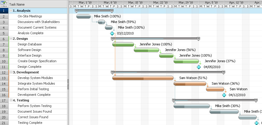
Gantt charts make it easy to visualize project management timelines by transforming task names, start dates, durations, and end dates into cascading horizontal bar charts.

An Excel Gantt chart

How to Create a Gantt chart in Excel

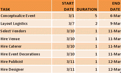
1. Create a Task Table

List each task in your project in start date order from beginning to end. Include the task name, start date, duration, and end date.

Make your list as complete as possible. Because of Excel’s limitations, adding steps or extending out may force you to reformat your entire chart.

2. Build a Bar Chart

On the top menu, select Insert, and then click on the Bar chart icon. When the drop-down menu appears, choose the flat Stacked Bar Chart, highlighted in yellow below. This will insert a blank chart onto your spreadsheet.

Add Start Date data.

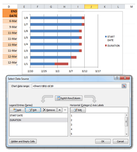
1. Position your mouse over the empty Excel chart and right click. Then, left click on Select Data. The Select Data Source window will appear.
2. Under Legend Entries (Series), click Add. This will take you to the Edit Series window.
3. Click in the empty Series name: form field first, then click on the table cell that reads Start Date.
4. Click on the icon at the end of the Series values field. The icon is a small spreadsheet with a red arrow (the lower icon). This will open the Edit Series window. Click on the first Start Date, 3/1 in my example, and drag your mouse down to the last Start Date. After the right dates are highlighted, click on the icon at the end of the Edit Series form. The window will close and the previous window will reopen. Select OK. Your start dates are now in the Gantt chart.

Next, add the Durations column using the same procedure you used to add the start dates.

1. Under Legend Entries (Series), click on Add.
2. Click in the empty Series name: form field first, then click on the table cell that reads Duration.
3. Click on the icon at the end of the Series values field. The icon is a small spreadsheet with a red arrow (the lower icon). This will open the Edit Series window. Click on the first Duration, it is 5 in my example, and drag your mouse down to the last Duration. After the durations are highlighted, click on the icon at the end of the Edit Series form. The window will close and the previous window will reopen. Select OK. Your durations are now in your Gantt chart.

Change the dates on the left side of the chart into a list of tasks.

1. Click on any bar in the chart, then right click, then open Select Data.
2. Under Horizontal (Category) Axis Labels, click on edit.
3. Using your mouse, highlight the names of your tasks. Be careful not to include the name of the column itself, Task.
4. Click on OK.
5. Click OK again.

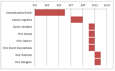
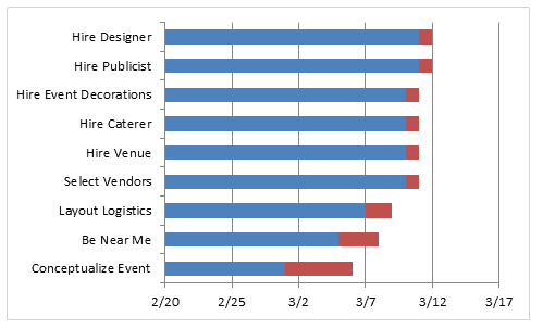
Your Gantt chart ought to look like this:

3. Format Your Gantt chart

What you have is a stacked bar chart. The starting dates are blue and the durations are red.

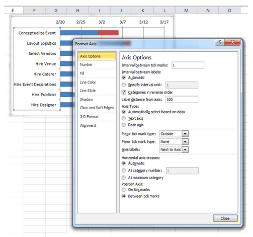
Notice your tasks are in reverse order. To fix this, click on the list of tasks to select them, then right click over the list and choose Format Axis. Select the checkbox Categories in reverse order and Close.

To give your Gantt chart more space delete the Start Date, Duration legend on the right. Select it with your mouse, then hit delete.

Hide the blue portions of each bar. Clicking on the blue part of any bar will select all of them. Then, right click and choose Format Data Series.

1. Click on Fill then select No fill.
2. Click on Border Color then select No line.

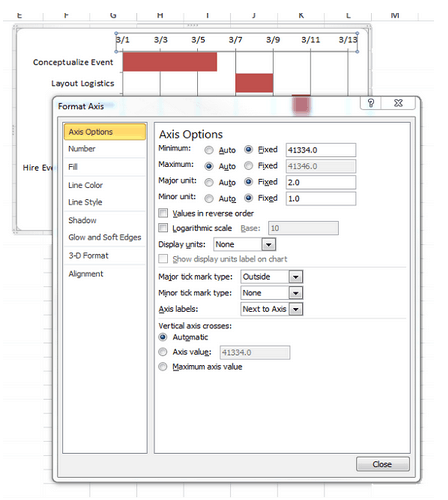
You’re almost finished. You just need to remove the empty white space at the start of your Gantt chart:

1. Click on the first Start Date in your data table. Right click over it, select Format Cells, then General. Write down the number you see. In my case it is 41334 Hit Cancel because you do not want to actually make or any change here.
2. In the Gantt chart, select the dates above the bars, right click and choose Format Axis.
3. Change Minimum to Fixed and enter the number you recorded.
4. Change Major unit to Fixed and enter 2, for every other day. You can play with this to see what works best for you.
5. Select Close.

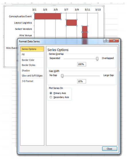
If you want to make your Gantt chart look a little nicer, remove most of the white space between the bars.

1. Click on the top red bar.
2. Right click and select Format Data Series.
3. Set Separated to 100% and Gap Width to 0%.

You are finished. Your Gantt chart should look like this:

This is a lot to remember.

While your Excel Gantt chart may look clean, it is not exactly serviceable.

• The chart does not resize when you add new tasks.
• It’s hard to read. There is no grid or daily labeling.
• You cannot change a start date, duration or end date and have the other values adjust automatically.
• You cannot share the chart with others or give them viewer, editor, or administrator status.
• You cannot publish an Excel Gantt chart as an interactive web page which your team members can read and update.

It is possible to create more complete Gantt charts in Excel, however, they are more complicated to setup and maintain. The things that make Gantt charts useful, sharable, and collaborative cannot be accomplished with Excel.